
Improving Disk Wiping Speed for Memory Wipes
Enterprise SSDs, multi-GPU label generation and a faster PoSE implementation. A ~14x speedup on persistent storage wipes.
Contents
Recap: in our last post, we introduced our work on memory wiping.
Memory wipes can be a useful tool when designing verification systems for AI workloads. Combined with network taps, recomputation and side-channel protections, they help to verify “completeness” of declared workloads.
In that post, we concluded that wiping memory on systems is slow due to slow disk write speeds, taking ~24 hours to wipe a system with 15 TB of storage. This post documents our follow-up work trying to improve this disk wiping process.
Background
Previously, we created a memory wiping prototype using the PoSE algorithm, which wiped RAM, HBM, and persistent storage. Read our last post for more detail on this.
We previously achieved very slow speeds wiping persistent storage. We used basic consumer SSDs for wiping, which had sustained disk write speeds of only 160–180 MB/s. This is despite advertised speeds of 8,500–14,000 MB/s, and the gap comes down to how NAND stores data.
Why are consumer SSDs slower than expected?
SSDs are made of many “NAND cells”. Each cell holds one bit (single-level cell, SLC), three bits (triple-level cell, TLC) or four bits (quad-level cell, QLC) depending on the design of the silicon.
More bits per cell is cheaper per GB but slower to write, so consumer drives use triple- or quad-level NAND cells, and hide the cost with a cache. We call this cache the pseudo-single-level-cell (pSLC) cache.
In the cache, each multi-level NAND cell is temporarily used to emulate a single-level cell by only using one of the levels. This cache can use a few GB to roughly a third of an empty drive, and shrinks as the drive fills.
Read this to learn more about NAND cell types.
Once the cache is exhausted, the drive writes directly to native TLC/QLC while compacting cached data in the background, and sustained speed falls to a fraction of the advertised figure.
Testing More Representative Drives
We decided to test wiping on drives that are more representative of datacentre storage.
What Drives?
Enterprise SSDs prioritise consistency (low variance in latency and throughput) over peak speed due to the sustained nature of datacentre workloads. They use faster 3D TLC or QLC NAND than consumer SSDs, and they don’t use the pSLC caching. This means their advertised write speeds are the same as their sustained write speeds.
NVL72 systems use E1.S form factor NVMe drives, which our own systems didn’t natively support, so we opted for U.2 NVMe drives. Both E1.S and U.2 form factors are NVMe over PCIe, so U.2 is representative enough for benchmarking.
Speeds
The drives we used for benchmarking were:
- 1x U.2 PCIe 5.0 NVMe drive with write speeds of 4000 MB/s
- 2x U.2 PCIe 3.0 NVMe drives with write speeds of ~2000 MB/s
These disk write speeds are faster than the label throughput of 126/245 MiB/s (CPU/GPU) that we achieved in our last post. Our next goal was to optimise label generation throughput.
Optimising Hash Generation for Disks
Our first idea for improving the wipe time of a large volume of disk storage was to parallelise the label generation process.
Using Multiple GPUs for Hash Generation
For machines that have multiple GPUs, we could use all of these GPUs (and potentially the CPU too) to produce labels for the disk space in parallel. This would be the first step of a system wipe, before the GPU’s own memory is wiped.
In theory, the label throughput should scale roughly linearly for each GPU added, up to the PCIe and backplane bandwidth limit.
Backplane Bandwidth
We want to ensure that the communication path isn’t the bottleneck when parallelising. Therefore, we need to understand the topology of the U.2 drive bays connecting to the server.
The following diagram shows a simplified topology of GPUs to NVMe drives in the front drive bays of a server. We expect this topology to be fairly standard for servers with multiple front-mount NVMe drives, including NVL72:
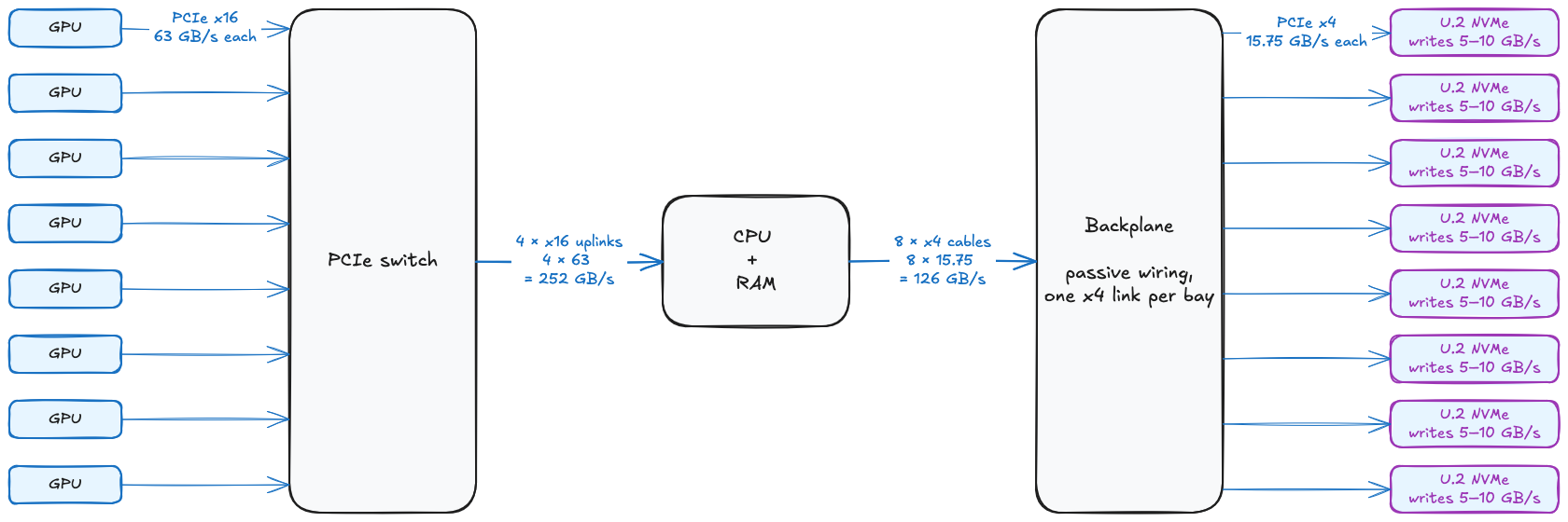
We estimate drive write speeds in the range of 5–10 GB/s, assuming most datacenters will be using high speed PCIe Gen5 drives with write speeds in the region of 10 GB/s, but also include a conservative lower bound of 5 GB/s for PCIe Gen4 drives.
Using our measured hash throughput of 244.5 MiB/s for one GPU, we get roughly 2 GB/s total label output for 8 GPUs. This is nowhere near saturating even the write speed of a single drive, let alone the bandwidth of any section of the path from GPU to drive.

Recap: Why multiple GPUs don’t break the security requirement
The security condition , explained in full in our last post, requires that the number of hashes required to recompute a robust label is more than a cheating prover could perform in the round trip time. Even though parallelising across multiple GPUs increases label throughput, it doesn’t break this requirement.
The relevant rate is the fastest single sequential chain an adversary can run, not their aggregate throughput. Adding GPUs to the fill doesn’t increase the sequential generation speed.
By contrast, filling is very parallel: each chunk’s graph is independent, so N GPUs fill N chunks concurrently. Multi-GPU generation therefore scales the fill linearly.
Multi-GPU Benchmark
To turn our above estimate into measured numbers, we built a benchmark tool that performs a real, full-disk wipe driven by the GPUs and reports the throughput it achieves. It reuses the exact same graph-labeling code as the RAM and HBM memory wipes from our last post, just adding the plumbing needed to write those labels onto a physical drive.
The Write Path
For each GPU the loop is:
- Host requests a block of labels and loads kernels
- Generate a block of labels into GPU memory
- Copy this block back to host RAM
- Write it straight to disk using
O_DIRECTsequential writes (bypasses OS page cache)
This is repeated, streaming blocks across every sector of the drive. As expected from the last post, label generation (2) is the bottleneck: the copy-back and disk write together only account for a small fraction of the time. Therefore, label generation becomes the thing to parallelise.
Splitting the Work across GPUs and disks
The tool exposes a fundamental parameter: how many GPUs team up on each disk. This covers the following options:
- One GPU per disk: every GPU writes to its own drive, so with N disks you wipe N in parallel
- Several GPUs per disk: the GPUs split a single drive into separate sector ranges and fill them concurrently, finishing one disk at a time.
- Anything in between (e.g. four GPUs across two disks, two GPUs per disk)
Crucially, the way we split the work never actually changes the bytes written. Each label depends only on the session seed and the label’s absolute position on the disk, so a disk filled by four GPUs has identical contents to the same disk filled by one. This allows us to improve speed without affecting the algorithm’s properties.
Confirming the Wipe
The tool reads a sample of labels back off the disk after wipe and recomputes the expected value on the CPU, comparing the two. This is the same check a verifier’s challenge performs, without the network round trip.
Guardrails
A real wipe is destructive, so the tool currently only touches drives named explicitly at runtime, refuses anything mounted or holding the operating system, and prints exactly what it will overwrite before it starts. This has been implemented for benchmarking purposes, but a full solution should wipe every drive on the machine without guardrails.
Optimising our PoSE algorithm
During a profiled run of our multi-GPU benchmark using NVIDIA’s CUDA profiler, we noticed that neither of the resources we expected to be limiting were busy. HBM throughput sat at 5% of peak and SM (compute) throughput at 19%, while L2 cache throughput was at 70%. The GPU was spending a significant portion of time waiting.
Two causes, and their fixes:
- Threads waiting for each other: Our original PoSE implementation used 8 groups of 32 threads (256 threads total) on the GPU per chunk. Every step of the wipe ended with a checkpoint where the whole group of threads waited for its slowest member. Most steps only had work for a few threads, so the rest just stood at the checkpoint. We gave each 32-thread group its own independent job, so no group ever waits on another. Eight times as many jobs run at once, each one smaller.
- Writing one byte at a time: Each 32-byte label was written as 32 separate one-byte writes, and the GPU’s cache treats each one as its own transaction. This flooded the cache with 16x more traffic than needed while the main memory sat idle. Write each label as two 16-byte chunks instead of 32 single bytes (16 bytes is the widest single memory instruction a CUDA thread has).
Every byte that lands on the disk is identical to before, only how they get there changed. This means labels and proof are unaffected, verified by comparing samples from the optimised implementation against labels independently recomputed on the CPU using the original code.
These optimisations sped up our single-GPU label generation throughput by ~3.3x on an H200, from 185 MiB/s to 620 MiB/s per GPU! (185 MiB/s is our H200 disk wipe speed, differing from our 244.5 MiB/s label generation throughput from our last post.)
Caveat: it uses more runtime memory
A downside to the optimised implementation is that it requires more memory to run (25 GiB). If used to wipe HBM, it means that 25 GiB of the HBM is supposedly wiped but isn’t attested. Fortunately, there are various solutions:
Wipe SSDs and RAM with the new implementation, then wipe the HBM later with the previous implementation.
Wipe in passes on the HBM. Another interesting option would be to use the new implementation on HBM but wipe in passes, meaning:
- Wipe all HBM but the reserved 25 GiB on first pass
- Reduce required memory to 2.5 GiB and wipe the remaining 22.5 GiB
- … Repeat until only a negligible amount of unattested memory remains
This would mean that the majority of HBM would be wiped at full speed, and only a small remaining amount would be wiped at slower speeds as allocated runtime memory is reduced. We have yet to prototype this approach but may in the future.
Results
We ran the benchmark on our HPE Cray XD670 server, with the following specs:
- CPUs: 2x Intel Xeon Platinum 8462Y+ 32 cores (64T) @ 4.10GHz
- GPUs: 8x NVIDIA H100 SXM
- RAM: 2TB DDR5
Figure 3 shows the results of each benchmark run (the full results table can be found in the appendix):
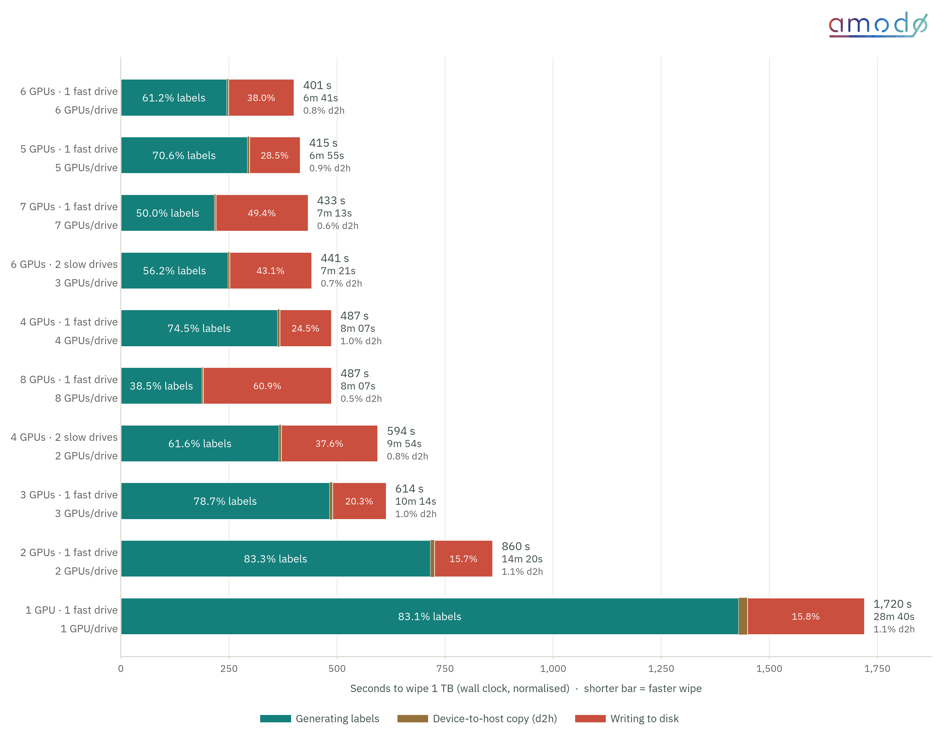
The fastest wipe throughput we achieved was with 6 GPUs wiping 1 fast drive, at a rate of 6 minutes 41 s per TB wiped. This is roughly a 14x speedup from our last post, due to both using a faster enterprise SSD, but also our algorithm improvements.
Figure 4 shows how aggregate throughput to one drive scales with GPUs added:
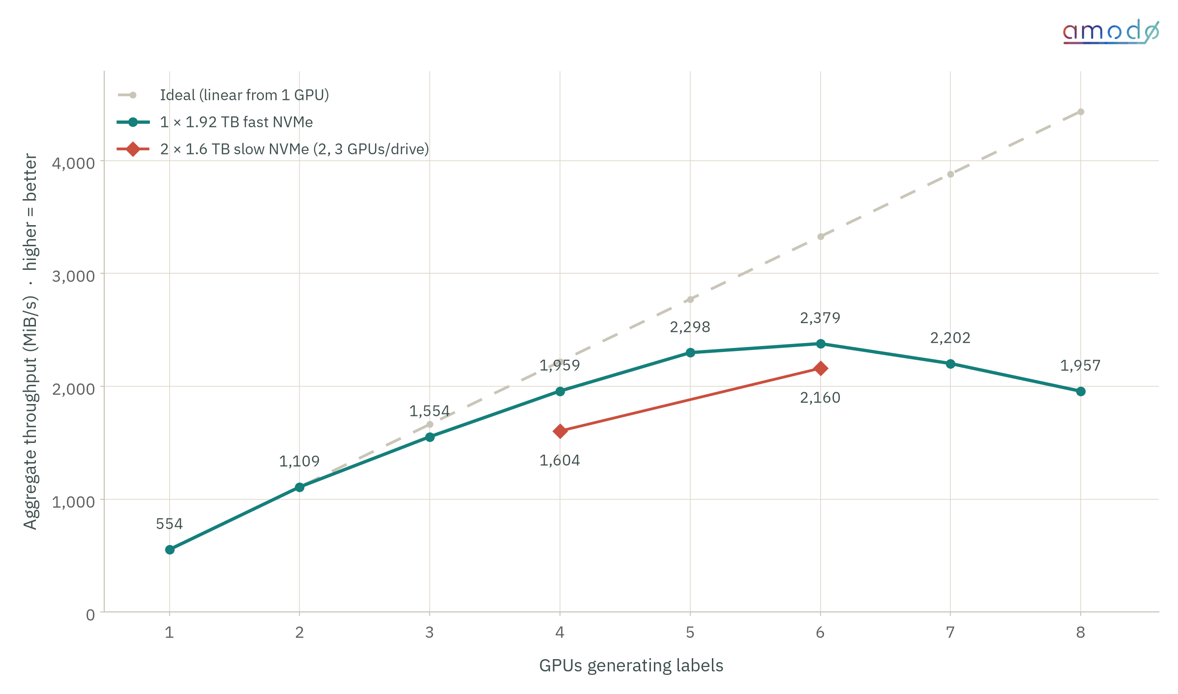
The aggregate throughput increases up to a peak at 6 GPUs, then degrades past this point. The reason for this is congestion on the write path, rather than GPU label generation (which stays roughly constant).
When multiple GPUs write to the same drive at once they block each other, even though the disk never reaches its rated write ceiling. The rating assumes a single device or process writing to the disk, and concurrent writers don’t get to share the full number between them.
This means the optimal way to wipe multiple drives in parallel is to parallelise multiple GPUs to multiple disks at a time, rather than “piling” all GPUs onto one disk at a time, wiping each disk sequentially.
Extrapolating Results to a GB200 NVL72 System
Using our benchmark results, we estimate that a single B200 GPU would achieve ~840 MiB/s label throughput with our current implementation. See the appendix for our calculation.
We have 30.72 TB drive space to wipe per tray in a GB200 NVL72 system (based on filling all 8 bays per tray with a 3.84 TB E1.S SSD).
Scaling the estimated 840 MiB/s for one B200 GPU to 4x GPUs we get 3350 MiB/s, and we can work out an estimate for how long it would take to wipe 30.72 TB of drive space at this throughput as:
If we wipe each of these trays in parallel, using each tray’s 4x GPUs to wipe its own persistent storage, we would wipe the rack’s total ~553 TB of persistent storage in ~2.5 hours, which is much faster than suggested in our last post.
Note: this is an estimate based on the assumption that Blackwell GPUs are somewhere in the region of our estimated 840 MiB/s label throughput. This would depend on whether the whole rack’s compute can be allocated to wiping simultaneously, the speed and size of the actual drives, etc.
PoSE is the current bottleneck
Looking back at Figure 1, we see that our hardware bottleneck is drive write speeds. If we take our lower bound of 5 GB/s write speed per drive (justified earlier), we get an aggregate drive write of 40 GB/s for 8 drives.
PoSE currently doesn’t generate labels anywhere close to fully saturating these values, but we can calculate how long an NVL72 tray wipe would take if PoSE (or another wiping algorithm) could saturate these throughputs:
- Best case:
- Worst case:
Again, if each of these trays is wiped in parallel, we could wipe the whole NVL72 rack in ~6–13 minutes. This is the hardware limit with current drive speeds, so to saturate this we need to improve the speed of the PoSE algorithm.
Conclusions and Future Work
Disk wiping speed is no longer limited by the hardware in our testing. Moving from consumer SSDs to enterprise U.2 drives removed the pSLC cache problem, and spreading label generation across GPUs and optimising our implementation gave us ~3.3x more throughput per GPU. We achieved a ~14x speedup over our previous post: ~7 minutes per TB, versus ~1 hour 30 mins per TB. Extrapolated to a GB200 NVL72, we expect each tray’s four GPUs to wipe its 30.72 TB of storage in around 2.5 hours, and the whole rack in the same time if every tray wipes in parallel.
We need to close the gap between label generation and enterprise SSD write speed, either by making PoSE substantially faster, or by finding another wiping algorithm that can saturate the write path.
If you or your team can help accelerate the pace of algorithmic improvement in PoSE, please contact us!
Pieces are still needed to turn memory wipes into a complete mechanism, including:
- Integrating the GPU disk wipe into a full system wipe
- We’re currently working on fully wiping BlueField DPUs
- Integrating memory wiping into a full verification scheme
- Shrinking the unwipeable memory
Appendix: Enterprise SSDs contain RAM
Part of the reason enterprise SSDs are able to achieve higher sustained write speeds is due to the fact that they have a small amount of onboard DRAM. Each drive has ~1 GB of DRAM per 1 TB of NAND. Assuming an NVL72 system that saturates 8 drive bays with 3.84 TB SSDs, we have 30.72 TB of NAND, therefore ~30 GB of DRAM per tray, totalling 540 GB per rack. Unfortunately for a memory wiping scheme, this means 540 GB more memory that needs to be wiped.
The DRAM typically contains:
| Contents | Details |
|---|---|
| Logical-to-physical mapping table | Maps host logical block addresses (LBAs) to physical NAND pages |
| Metadata | Wear-levelling stats, bad-block lists |
| Small write buffer | Typically 10s of MB of user data in flight before it’s committed to NAND |
Table 1. Typical contents of an enterprise SSD's onboard DRAM.
Unfortunately, the DRAM normally sits on the controller’s private bus, so NVMe/SATA commands give the host no way to read or write it directly. An exception is that, in rare cases, some NVMe drives expose a Controller Memory Buffer (CMB) (few MB to 256 MB) or Persistent Memory Region (1–8 GB, though only on niche MRAM/FPGA accelerators rather than mainstream SSDs). This is a slice of DRAM that the host can map and use. An exposed slice like this should be relatively straightforward for us to wipe.
Beyond this, we would likely need custom firmware or physical probing of the chips to wipe it, which a cheating prover would also need. We decided this is out of scope for this specific experiment, but it remains a necessary piece of future work.
Appendix: Results table
| Run | GPUs / drive | Storage (TiB) | Wall clock | s / TB | Aggregate (MiB/s) | Per-GPU (MiB/s) | Label % | d2h % | Write % |
|---|---|---|---|---|---|---|---|---|---|
| 1 GPU · 1 fast drive | 1 | 1.75 | 55m 03s | 1,720 | 554.5 | 554.5 | 83.1 | 1.1 | 15.8 |
| 2 GPUs · 1 fast drive | 2 | 1.75 | 27m 32s | 860 | 1,108.9 | 555.5 | 83.3 | 1.1 | 15.7 |
| 3 GPUs · 1 fast drive | 3 | 1.75 | 19m 39s | 614 | 1,553.9 | 521.3 | 78.7 | 1.0 | 20.3 |
| 4 GPUs · 1 fast drive | 4 | 1.75 | 15m 35s | 487 | 1,958.7 | 494.7 | 74.5 | 1.0 | 24.5 |
| 5 GPUs · 1 fast drive | 5 | 1.75 | 13m 17s | 415 | 2,298.5 | 467.3 | 70.6 | 0.9 | 28.5 |
| 6 GPUs · 1 fast drive | 6 | 1.75 | 12m 50s | 401 | 2,378.7 | 406.1 | 61.2 | 0.8 | 38.0 |
| 7 GPUs · 1 fast drive | 7 | 1.75 | 13m 52s | 433 | 2,202.4 | 331.2 | 50.0 | 0.6 | 49.4 |
| 4 GPUs · 2 slow drives | 2 | 2.91 | 31m 42s | 594 | 1,604.4 | 409.9 | 61.6 | 0.8 | 37.6 |
| 6 GPUs · 2 slow drives | 3 | 2.91 | 23m 33s | 441 | 2,160.3 | 371.5 | 56.2 | 0.7 | 43.1 |
| 8 GPUs · 1 fast drive | 8 | 1.75 | 15m 36s | 487 | 1,957.1 | 255.4 | 38.5 | 0.5 | 60.9 |
Table 2. Full benchmark results after algorithmic optimisation. "d2h" is the device-to-host copy.
Appendix: Results before algorithmic optimisation
Note: the remaining percentage after label + write is the device-to-host copy time, which is 0.3% for every run.
| Run | Storage (TiB) | Wall clock | Aggregate (MiB/s) | Per-GPU (MiB/s) | Label % | Write % |
|---|---|---|---|---|---|---|
| 2 GPUs, 1 drive | 1.46 | 1h 17m | 330.2 | 165.5 | 90.9 | 8.8 |
| 4 GPUs, 1 drive | 1.75 | 46m 25s | 657.4 | 167.1 | 91.8 | 7.8 |
| 4 GPUs, 2 drives · 2 GPUs/drive | 2.91 | 1h 17m | 657.9 | 165.5 | 90.9 | 8.8 |
| 4 GPUs, 2 drives · 4 GPUs/drive (seq.) | 2.91 | 1h 20m | 634.0 | 159.2 | 87.5 | 12.2 |
| 6 GPUs, 2 drives · 3 GPUs/drive | 2.91 | 52m 10s | 974.9 | 163.8 | 90.0 | 9.7 |
| 6 GPUs, 1 drive | 1.46 | 27m 41s | 918.5 | 154.5 | 85.2 | 14.5 |
| 7 GPUs, 2 drives · 7 GPUs/drive (seq.) | 2.91 | 47m 58s | 1060.4 | 152.5 | 84.0 | 15.7 |
Table 3. Benchmark results before the thread-grouping and 16-byte write optimisations.
The following graph shows the results of each benchmark run before implementing our thread size and 16 byte write optimisations:
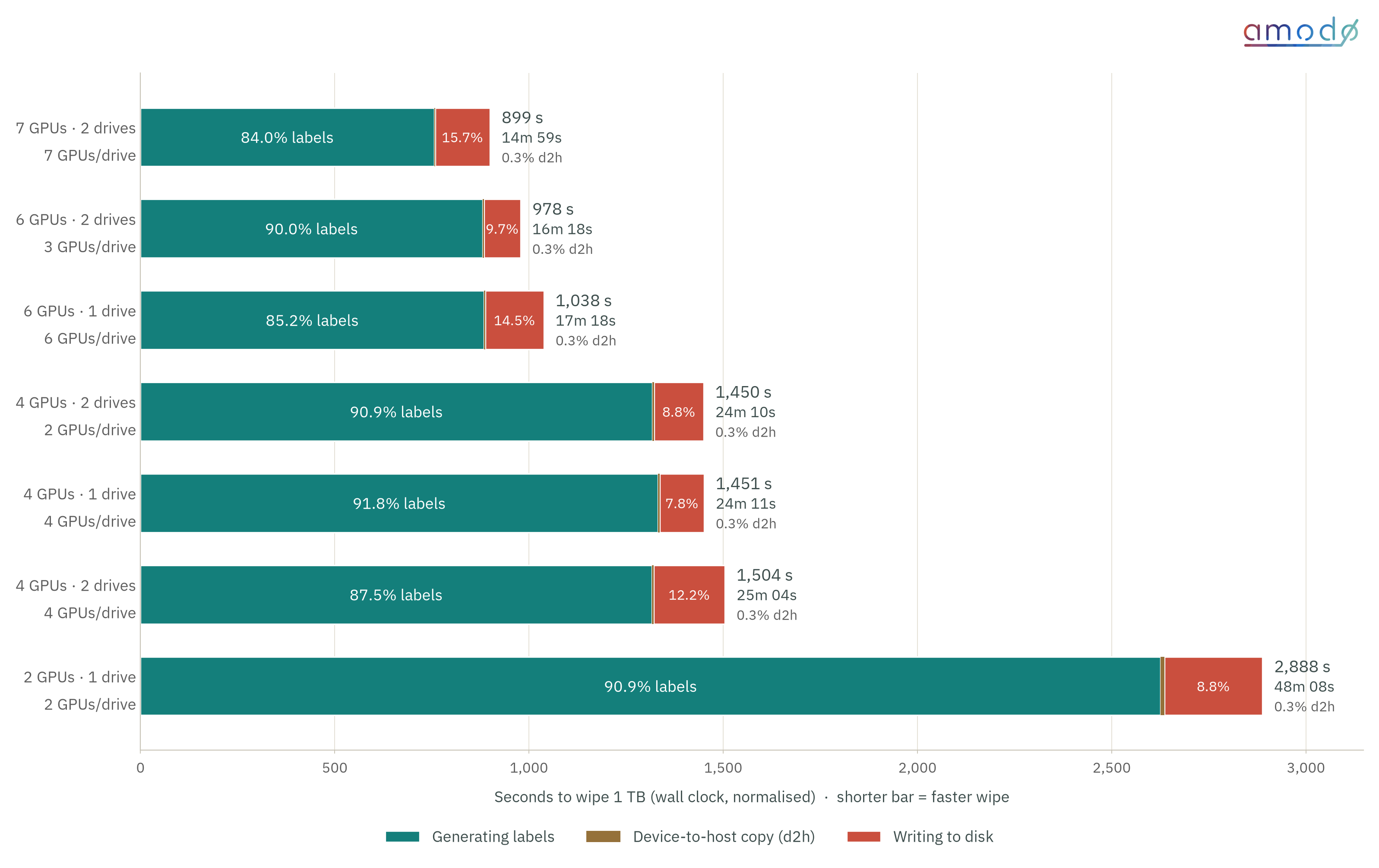
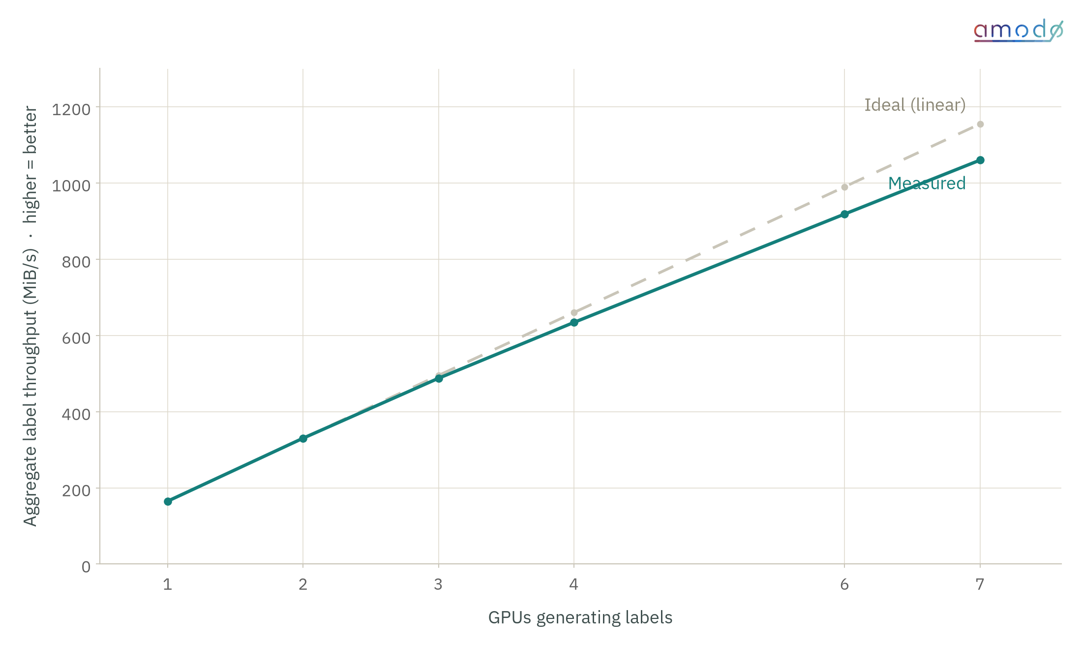
The graph above shows how aggregate label throughput grows as more GPUs are added to generate labels. It scales close to linearly, but not quite. The reason for this isn’t actually the GPU label generation, which stays roughly constant across every run, but instead the write path. When multiple GPUs write to the same drive at once they interfere with each other, even though the disk never reaches its rated write ceiling. The rating assumes a single device or process writing to the disk, and concurrent writers don’t get to share the full number between them.
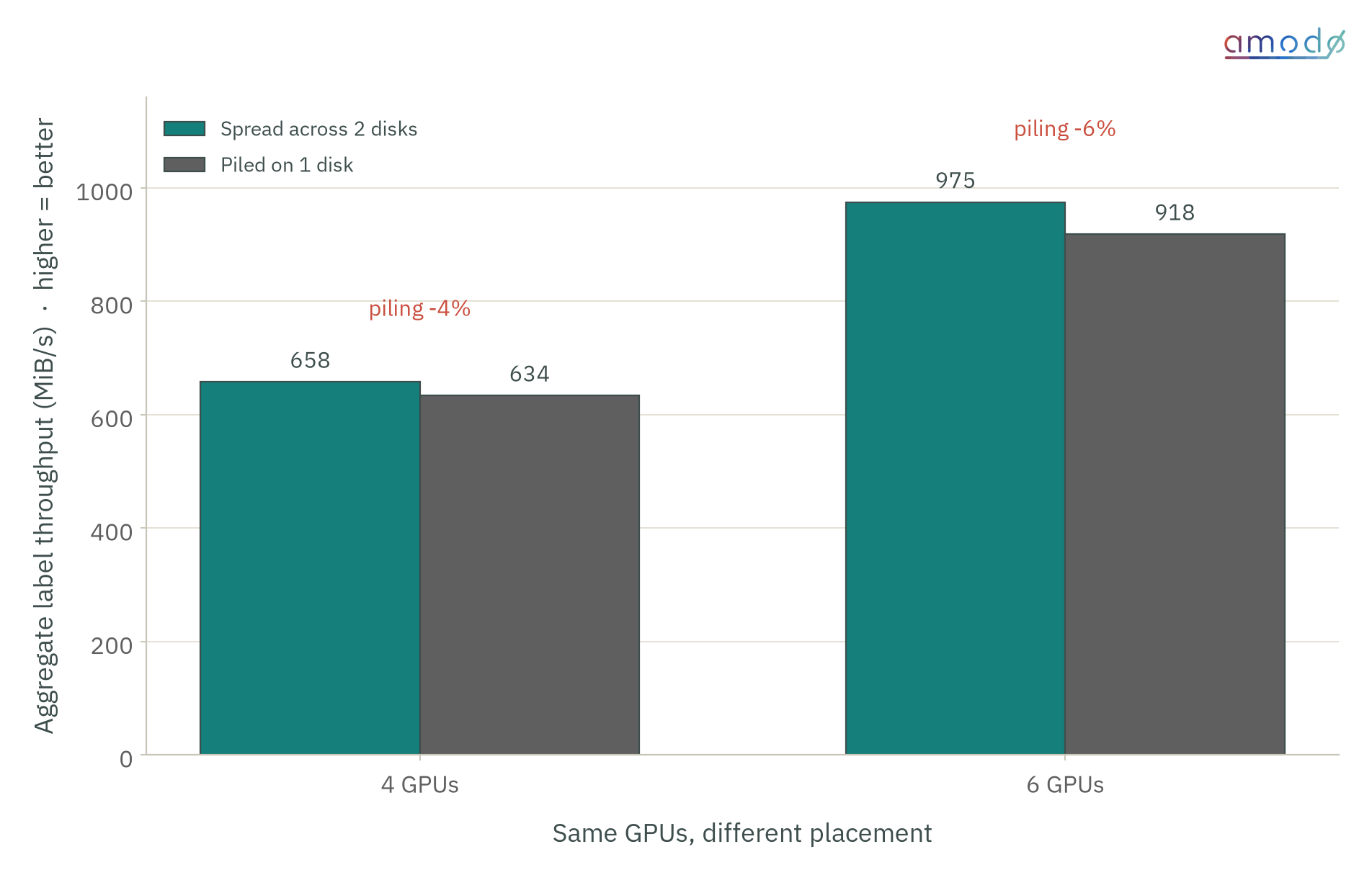
The diagram above also shows the same effect, comparing GPUs spread across two disks in parallel against all GPUs “piled” on one disk and wiped sequentially. The overhead is fairly small at this scale, but it’s still large enough that parallelising GPUs across multiple drives is the better default, rather than piling everything onto one drive at a time.
Appendix: Extrapolating PoSE speeds to B200
Time per MiB is a cycle-bound term plus a bandwidth-bound term:
Two GPUs, two unknowns. The H100 SXM is 132 SMs at 1980 MHz with 3.35 TB/s; the H200 NVL is 132 SMs at 1785 MHz with 4.8 TB/s.
Solving:
Extrapolation to B200 (148 SMs, 1900 MHz placeholder, 8.0 TB/s):
Estimate: about 840 MiB/s per B200, roughly 1.35× the H200.