Memory Wipes - Performance Analysis

Memory wipes can be a useful tool when designing verification systems for AI workloads. Combined with network taps, recomputation and side-channel protections, they help to verify “completeness” of declared workloads.

Background

For our purposes, memory will refer to anything that stores information: registers, caches, HBM, RAM, SSD, etc.

A cluster is operated by the prover and checked by the verifier. A memory wipe involves the prover wiping all memory, and then a verifier ensuring that the prover has fully overwritten its memory, with no information persisted across the wipe. In practice, a small amount of memory may be unwipeable. We want to achieve that without the verifier needing to trust the prover’s hardware; we’d also like this operation to take ~minutes rather than hours or days.

Our approach is for the verifier to give the prover a set of random numbers to write to memory. The only way the prover can read them back to the verifier is if they filled their entire memory with those numbers, meaning nothing else can be stored there. This is a Proof of Secure Erasure (PoSE).

Simple in theory

But in practice, memory wipes aren’t trivial. Here are some of the initial challenges we found when experimenting with memory wipes on a tray of H200s.

Devices abstract memory for the user

The main challenge with implementing this is that modern devices don’t normally let you write directly to memory; that is the domain of the OS and the CPU’s memory management unit (MMU). The OS and the MMU work together to manage the RAM such that when an application starts it believes it has access to all available memory as defined by the OS. This is often larger than the actual available memory; this is achieved using virtual memory and memory maps.

Both physical memory and virtual memory is split into chunks known as pages, these pages are then managed by the MMU using a memory map. The memory map acts as a lookup table between the virtual and the physical memory.

When the user allocates some memory, it is first assigned an address in the virtual memory space inside a page, and the OS passes the request onto the MMU, which then assigns it to an available space in a physical page and location.

If a new page needs to be created but the RAM is currently full, the MMU returns a fault to the OS, and the OS will request the MMU evict a page provided by the OS to free the memory. Later, if the user asks for data that is not currently in the RAM but is now on disk, the same process applies, with the OS nominating one or more pages to be evicted and the user’s page is then brought in.

/dev/mem

The main way to work around this limitation is to use memory mapping (mmap()) on a special virtual device in Linux called “/dev/mem” which represents the raw physical memory. Unfortunately, most standard builds of Linux have this disabled for security reasons — it’s easily abused by malware as it allows direct read and write access to the kernel’s own memory — but it can be enabled when building the OS from scratch. This allows us to access physical memory, but we still find our process being halted, having our memory paged, or even Linux terminating our process if it decides it needs its memory back.

The correct way to solve this is at the lowest OS level (“ring 0”). The program should be executed as a kernel, which will give it privileged access to the system to allow us to disable paging to disk for our memory. However, if the OS requires more memory but we have consumed it all, the OS will simply crash.

Wiping everything

How do we maximise the amount of memory we wipe? Ideally, we would wipe every bit of memory, disk, HBM etc., but this isn’t trivial.

We should not overwrite drivers and OS, which means there will always be some memory that we’ve not wiped. To minimise the amount of memory we don’t wipe we start with a stripped-back OS with as little overhead as possible. We only include the components we need to perform the wiping. Once memory wiping is complete, we can reinstall/initialise a full OS.

Wiping it all at once

The last challenge is a constraint on the system: all data must be simultaneously wiped across the system. If we were to wipe one disk, then the next, an attacker could simply move the data between the disks. The same goes for the compute trays, where it may not be possible to observe the inter-tray communications; data could simply be moved between devices.

On a single device, this problem is easier to solve as we simply have to label all memory and disk space before we perform the challenges. We then randomly challenge data from memory and disk such that an attacker cannot guess where we will request data from next.

There are lots of bits of memory

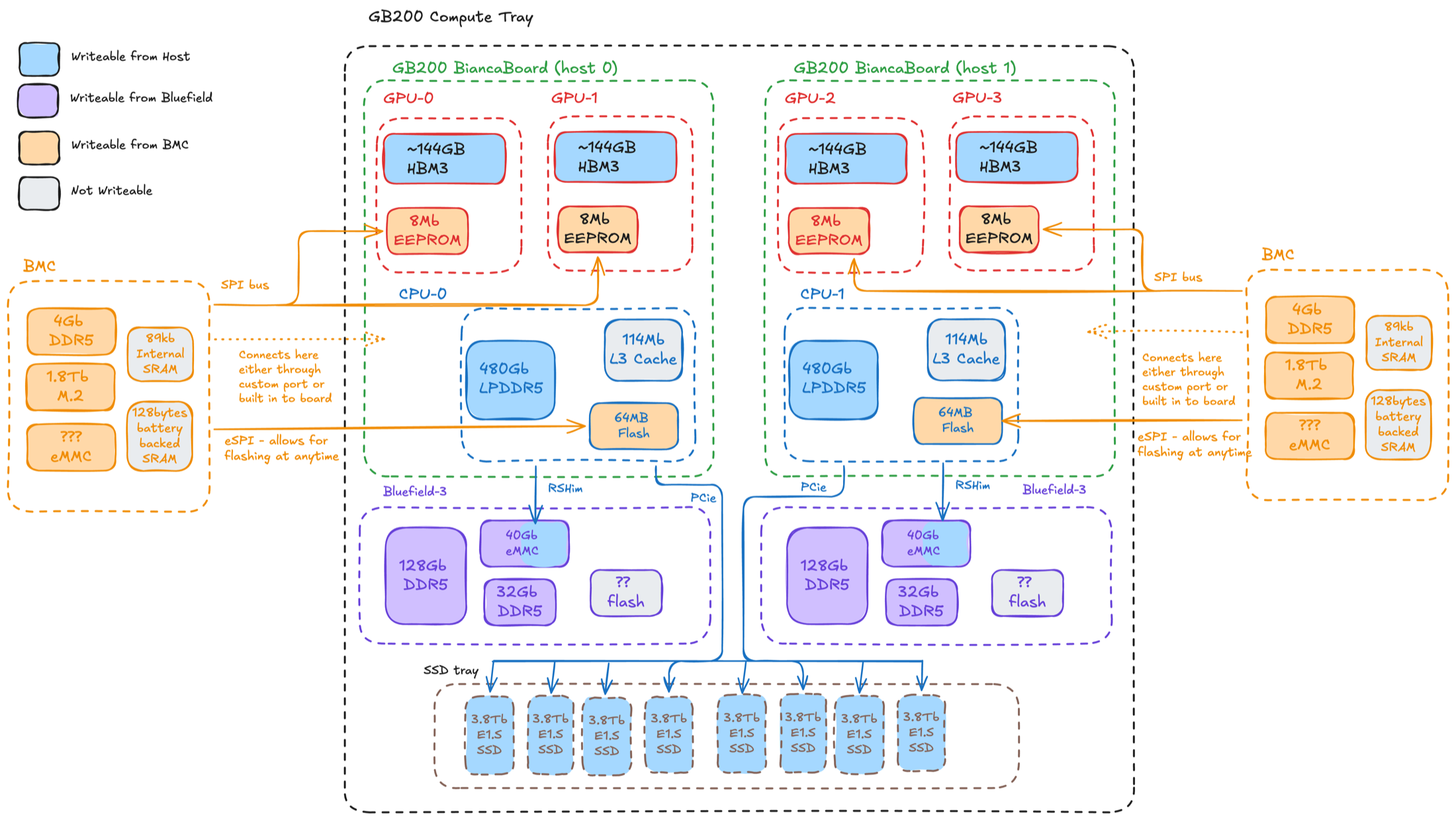
These are estimates of where all of the memory is on a GB200 system, and how much is non-wipeable (e.g. due to drivers and keys).

Device	Store	Memory per device	Rack total	Non-wipeable memory
GPU	HBM3	192 GB	≈ 13.8 TB	<100MB (drivers)
	firmware EEPROM	8 MB	≈ 576 MB	<1MB (keys)
Host	DRAM (LPDDR5X)	480 GB	≈ 17 TB	<50GB (usable capacity)
	BIOS flash	64 MB	≈ 2.3 GB	<1MB (keys)
	M.2 SSD	1.8 TB	≈ 32 TB	<400GB (usable capacity)
	L3 cache	114 MB	≈ 4 GB	114MB (cache)
BMC	DRAM (DDR)	4 GB	≈ 72 GB	<128MB (OS)
	internal SRAM	89 KB	≈ 1.6 MB	89 KB (next boot)
	battery-backed SRAM	128 B	≈ 2.3 KB	128 B (next boot)
DPU	DRAM (DDR5)	32 GB	≈ 1.1 TB	<128MB (OS)
	on-board SSD	128 GB	≈ 4.6 TB	<60GB (usable capacity)
	eMMC (boot + OS)	40 GB	≈ 1.4 TB	<8G (usable capacity)
Tray	E1.S NVMe SSD	3.84 TB	≈ 553 TB	<700GB (usable capacity)
Various	One-time-programmable	—	—	<10MB (keys)

Table 1. Estimated memory stores on a GB200 system and how much of each is non-wipeable.

Proof of Secure Erasure

The PoSE protocol relies on storing known data on the prover and then having the verifier challenge that data at random to ensure that the prover has stored it. There are two ways proposed to do this: you either stream to the device enough random data to fill all available memory, or propose an algorithm for calculating the data on the device from a random key.

Fill	The prover writes data to every location to be erased.
Challenge	The verifier requests the contents of randomly chosen locations under a timeout and checks them against the expected values. The timeout is small enough that the prover cannot have recomputed the data, or retrieved it from another device.

Pros and cons of streaming versus generating the data on device:

• Streaming. Network bandwidth becomes the bottleneck. Regular links operate at a 400 Gb/s interface. That means it would take 2-3 hours to move the 500TB required at rack scale.
• On device. This removes the network link from the critical path, at the cost of doing more computations on the device being erased.

We chose to generate the fill on the device using the approach described in Bursuc et al. (arXiv:2401.06626). Two things that we want to ensure:

• The prover is able to quickly produce the data for the challenges, and the process is repeatable on the verifier such that the verifier can cross-check.
• The verifier shouldn’t have to store all the information the prover is storing.

We achieve this by constructing a directed acyclic graph (DAG) — a set of nodes joined by one-way edges with no cycles (a graph has no cycles if there is no path from a node back to itself). One node maps to each memory location to be filled. Each node n is given a label $L(n)$, the value to be written to its location:

$$L(n) = H\!\left(n \,\|\, L(p_1) \,\|\, \ldots \,\|\, L(p_k)\right)$$

where H is a hash function, $p_1 \ldots p_k$ are the nodes with edges into n (its parents), and $\|$ is concatenation. A root node with no parents takes $L(n) = H(n)$. A node’s label depends on its parents’ labels, so no label can be produced without first producing everything upstream of it.

The verifier sends the seed and pre-computes the labels it intends to challenge. It knows the correct answer for any location without holding the whole graph.

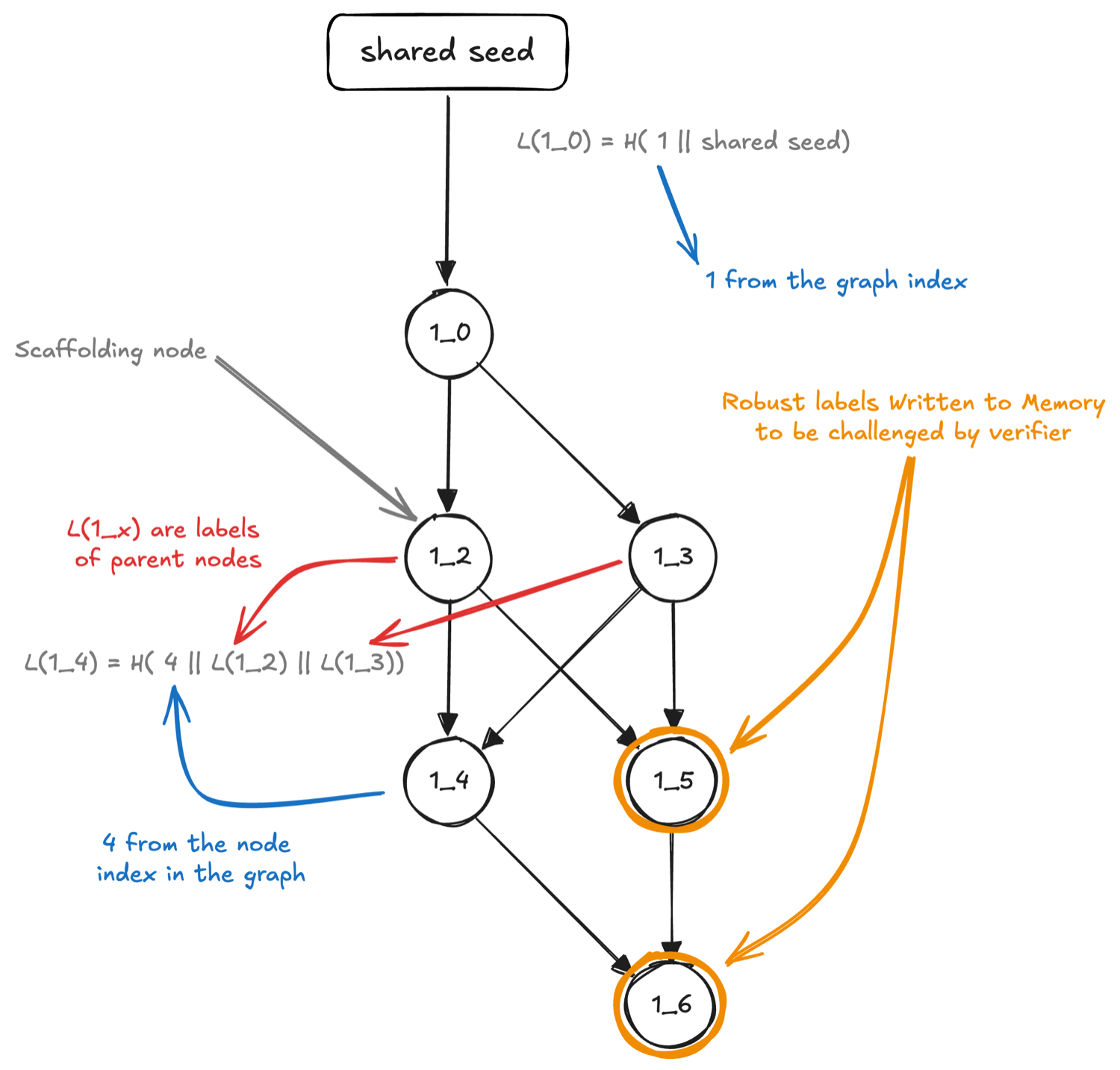
In practice, the graphs are constructed in a more sophisticated way (see the paper for technical details), which gives a few properties:

• In-place construction: the graphs can be built by self-overwriting so that little additional memory is required.
• Depth robustness: labels in the graph can be differentially easy/hard to recalculate. Trivial example: the first label only requires one hash to derive from the initial seed. A cheating prover could discard labels that would be easy to recompute at challenge time. To solve this, we only use the labels that are sufficiently hard to calculate from the previously used labels (e.g. we would not pick the very first label).

There are many labels that are calculated as part of building the robust labels — we call these extra labels “scaffolding”. They exist transiently during the calculation of the labels for robust nodes.

Scratch is the memory space that is needed to provide intermediate calculations. Ideally this is small, as it is difficult to wipe this section of memory itself, given that it is used by the algorithm during the wiping process.

Challenge and round-trip time

As outlined above, the verifier requests data from certain locations in memory, which contain robust labels. The verifier enforces a timeout on responses, which should give the prover enough time to retrieve the correct label but not enough time to recompute it — showing that it must have been stored by the prover.

The “round-trip time” of the communication link is a reasonable upper bound for how long the prover would have to try to recompute one of the labels. The depth of the graph is set such that this recomputation is not possible before the timeout.

The time to recompute a robust label must be more than the round-trip time (RTT) for the system to be “secure”. We define $q$ as the number of hashes a cheater can compute in the RTT, and $\gamma$ as the minimum number of hashes that must be recalculated to recompute a robust label.

We calculate $q$ and $\gamma$ for our system in the experiments below.

Experiments

Demonstrating the algorithm on a Raspberry Pi

To test the setup we ran the basic algorithm on a Raspberry Pi 5, erasing its RAM and a connected SSD.

The first stage was our own custom image, stripped as far back as possible — as much disabled at build time as we could manage. We didn’t even include display drivers; we attached a UART for a live debug stream. Rather than write the image to an SD card, we network-booted it, which gave two advantages: the OS and its overhead lived in one place instead of being managed separately, and a rebuild-and-reboot redelivered the image automatically.

The erasure daemon itself is written in C and built into the kernel, sharing its graph and hash libraries with the verifier (written in Rust) so both compute the same graph and labels.

The most complex part was managing which memory could and could not be erased: get it wrong and the result was the OS’s out-of-memory killer terminating the process, a segmentation fault, or a complete crash from trampling the OS’s own memory.

Once a simple single-threaded version was wiping >1,900 MB of the 2 GB of RAM and all of the attached NVMe — albeit slowly — we set about optimising it through:

• In-place labelling: you store the node ID and its list of parents into the location that the label will go. When you generate the hash, you overwrite that information because you wrote it into the place where the label was meant to be — so you didn’t use any scratch to generate that hash.
• Multi-threading: using multiple cores for different graph segments.
• Single Instruction, Multiple Data (SIMD): inline parallelising of identical mathematical operations, achieving multiple operations at the cost of a single instruction.

The Pi’s Broadcom VideoCore is not CUDA-capable, so there is no GPU path here. The GPU and CPU share memory, which we wipe regardless.

Hash selection

The hash function H does not need to be cryptographically strong, thanks to the graph structure and timed-challenge scheme. The one requirement is that H behaves as a random oracle: knowing one output gives no way to produce another without actually performing the calculation.

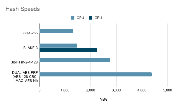
It is preferable that the hash function is as fast as possible, to keep wipe times as small as possible. The algorithm requires us to hash small inputs efficiently, which is not typically what hashing algorithms are optimised for. We benchmarked several hashing algorithms on small inputs (56–192 bytes) on our hardware (CPU: AMD EPYC 9335, 32-core; GPU: NVIDIA H200 NVL).

Algorithm	Device	Hash rate	Label size	Output datarate
BLAKE3	EPYC 9335 (CPU)	7.95 × 10⁶ h/s	32 B	1,456 MB/s
SHA256	EPYC 9335 (CPU)	7.19 × 10⁶ h/s	32 B	1,317 MB/s
BLAKE3	H200 NVL (GPU)	~1.23 × 10⁷ h/s	32 B	2,252 MB/s
DUAL-AES-PRF (AES-128-CBC-MAC, AES-NI)	EPYC 9335 (CPU)	40.9 × 10⁶ h/s	32 B	4,373 MB/s
SipHash-2-4-128	EPYC 9335 (CPU)	51.7 × 10⁶ h/s	16 B	2,760 MB/s

Table 2. Hash rates on small inputs (56–192 bytes) by algorithm and device.

Conclusions:

• BLAKE3 is the only algorithm that makes sense for use on the GPU. Its parallel nature makes it ideal for GPU-based computation.
• On the CPU, DUAL-AES-PRF and SipHash beat BLAKE3 and SHA. AES-NI and SipHash are much faster on short inputs, while BLAKE3 is comparatively slow.

Note on DUAL-AES-PRF: this is a pseudo-random function built from AES-128-CBC-MAC. It is not a cryptographic hash, but it meets the requirement for a random oracle that creates fixed-length digests.

We therefore use BLAKE3 on the GPU (for HBM) and Dual-AES-PRF on the CPU (for DRAM and SSDs).

Fill time and optimisation

To wipe some storage, we need to generate many more labels than would fit inside it, as many are discarded because they are not robust (see above). For example, in some tests we have had to generate ~2000× as many labels as would fit in the storage being wiped.

Let $N$ be the total number of labels required to calculate the whole scaffold to fill a region of storage. The time taken to fill the memory is:

$$t = \frac{N}{r}$$

where $r$ is the rate of hashes per second.

For a memory size of 130 GiB with 32-byte labels, we would need ~$4.4 \times 10^{9}$ robust labels. However, the scaffold means we actually need to calculate $9.1 \times 10^{12}$ labels — nearly 2084× more! With the measured Dual-AES-PRF rate of $40.9 \times 10^{6}$ h/s:

$$t = \frac{9.1 \times 10^{12}}{40.9 \times 10^{6}} \approx 61\ \text{hrs}$$

We can optimise this by “chunking” our memory and computing a graph for each chunk in parallel — so long as $q < \gamma$.

For these experiments, we assume an RTT of 1 ms. This is expected to be a safe overestimate:

• The retrieval of the data from memory should be ~100 ns.
• The high-speed networking equipment in frontier data centres is capable of switching traffic with only µs latency.

We can therefore calculate a budget for each of our hashing devices for the RAM:

$$q = 40.9 \times 10^{6}\ \text{hashes/s} \times 1 \times 10^{-3}\ \text{s} = 40{,}900\ \text{hashes}$$

For the system to be secure, we need $\gamma$ greater than this. (Reminder: $\gamma$ is the minimum number of hashes needed to recompute a robust label.) Our graph construction forces $\gamma$ to be a power of 2 — in our case $2^{16} = 65{,}536$, the smallest power of 2 greater than $q$. Due to the construction of the graph, the number of robust labels in each graph ($\mu$) equals $\gamma$.

We now split our memory into “chunks” and produce a graph that outputs at least $2^{16}$ robust labels. This has two main implications:

• Smaller $\mu$ means a shallower graph, so the scaffold per robust label shrinks ($\sim (\log_2 \mu)^2$), reducing wipe time.
• Per-thread scratch shrinks ($\propto 2^{\,n(\mu)}$), reducing memory use, which means a greater fraction of the memory can be wiped.

In addition, the GPU uses multiple threads per tree, calculating each node in each level of the tree simultaneously; this lets us use less scratch and better utilise the GPU.

Tested on our hardware, assuming an RTT of 1 ms and using a $\gamma$ of 65,536 for the RAM and a $\gamma$ of 32,768 for the GPU, using 32 CPU threads:

Device (Algorithm)	Memory to be wiped	Scratch used	Throughput (MiB/s)	Wipe time
RAM (Dual-AES-PRF)	120 GB	640 MiB	126.3	927 s
GPU (BLAKE-3)	140 GB	792 MiB	244.5	524 s

Table 3. Wipe performance with chunked graphs on our hardware (1 ms RTT, 32 CPU threads).

The wipe times here are much faster! Scaling these numbers to the sizes in a GB200 tray, total wipe time is 2565 s (43 minutes).

We benefit from AES-PRF being on the CPU and BLAKE3 being faster on the GPU, as this means we can constrain each separately — i.e. we prevent the GPU being used to cheat by recalculating hashes for the CPU RAM, and vice versa.

Challenge time

The secondary performance question is: how long does the challenge phase take?

During the challenge phase, the prover reads labels from random locations and returns them before the timeout. The access pattern must be unpredictable so the prover cannot store only the hashes it expects to be challenged. (We expect to have calculations for this shortly — watch this space!)

The slow part of the challenge phase is that the verifier needs to calculate all the labels it wishes to challenge. We have broken the graph into pieces, which allows the verifier to not perform any calculations for a tree that it will not challenge. This can also be managed by having the verifier calculate the labels while the erasure is happening, or even pre-compute them beforehand.

The disk problem

Most modern NVMe drives communicate via PCIe. PCIe 5 drives offer read/write speeds of between 8,500 MB/s and 14,000 MB/s. Most 1 TB drives will use around 30 GB of the disk as a fast cache. Data in this space can be accessed with the maximum throughput of the drive, which will attempt to keep recently used files in this area. However, the rest of the drive cannot be consistently accessed at these speeds.

We attempted to write hashes to fill our 1 TB drive, a PCIe 4×4 NVMe drive offering 4,000 MB/s of write speed. Initially, the disk performed at the advertised speed. However, after writing approximately 12 GiB of data the speed began to drop significantly. The write became unstable, fluctuating between 70–180 MiB/s. Writing a full 1 TB gave a final average write speed of 160 MiB/s — much lower than the advertised rate — taking ~1h 35 minutes.

This is the main ceiling on the performance of the algorithm on many types of hardware: scaling this up to a GB200 system with 15 TB of storage could take over 24 hrs to write the hashes. It may be possible to write to different drives in parallel to reduce this time. While newer PCIe 5/6 drives are likely to have better sustained speeds than our drive, we expect that the largest constraint on the system is the volume of disk space that needs to be erased.

Conclusions and future work

• We believe you can securely erase both RAM and GPU HBM in ~10s of minutes, even on hardware with lots of memory (e.g. GB200).
• Wiping high volumes of disk space causes a big slowdown. Large systems can take ~10s of hours to be wiped. Our next package of work will try to speed this up:
  • Assess the feasibility of writing to each disk separately, in parallel.
  • Use the GPU to generate the hashes for the disks if hash-generation speed becomes the bottleneck.
  • Investigate “partial” or “cumulative” wipes, to only need to wipe part of each system.
  • What data-centre architectures would allow the storage to be separate from the trays? How would a data centre look if this were the case, and what wiping strategies would you need?
• The amount of memory that cannot be wiped should be less than 1 GiB total, through the creation of a minimal Linux image. Further work is required to minimise the overhead of including the GPU drivers in the image, as well as how these images can be deployed to hardware (think memtest, for memory wiping!).
• Other devices in the data centre have memory, for example network switches (frontend, backend, management). How can we wipe their memory?
• Further benchmarking, especially varying $\gamma$, to see its impact on performance.