Example Schemes for Verifying High-Stakes AI Agreements

Introduction and framework

This post outlines some possible recomputation-based verification algorithms that we are trialling to verify AI model inference and pre-training. We bring together methods taken directly from others’ work and our own thinking.

We present these together as a precursor to sharing our current engineering work implementing and testing these schemes on our in-house hardware.

By “AI Verification” we mean two or more parties agreeing to some details of how AIs are trained or deployed. We refer to parties as:

• The Prover — the party performing the AI workloads and making the declarations.
• The Verifier — the party to whom the declarations are being made, and who verifies that they are correct.

We envisage these technical schemes being used in different verification scenarios:

• Government (prover) → Government (verifier)
• AI Developer (Lab) (prover) → Government (verifier)
• AI Developer (Lab) (prover) → AI Developer (Lab) (verifier) agreements
• AI Developer (Lab) (prover) → 3rd party (verifier) agreements

Whilst we have spent some time thinking about what these prover/verifier agreements might look like, this document focuses on the technical feasibility of verifying a workload running on an AI compute cluster.

Scope

Across our writings, we break down verifying workloads into two components: correctness and completeness.

• Correctness — the workloads that are being run and reported match the workloads that the prover declared they would be running.
• Completeness — all the workloads that the prover is running are being reported.

This post is on algorithms that check for correctness.

Technical schemes for workload verification

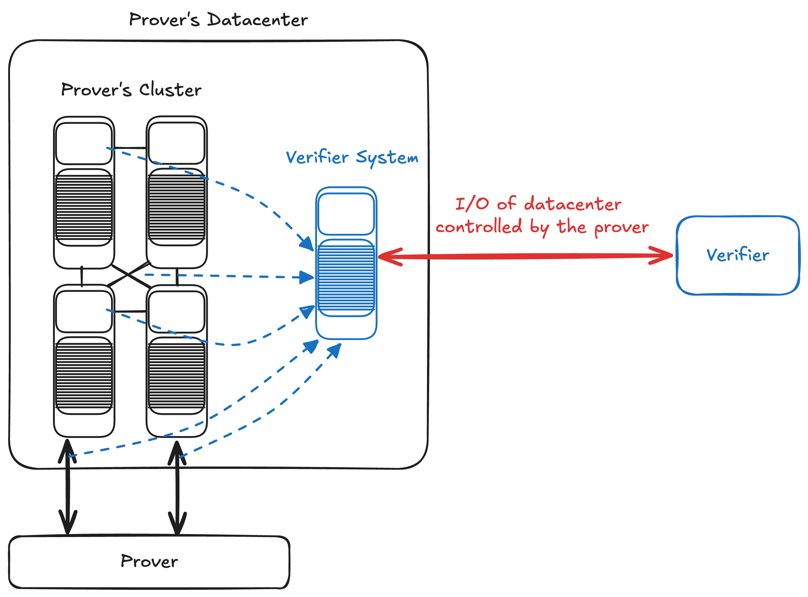
These schemes assume cooperation between the prover and the verifier, including the verifier installing a “recomputation server” in the prover’s data centre. In each example, the prover is providing some information to the verifier that they run on this recomputation server.

The basic intuition for how prover data is kept confidential is that the recomputation server is within the prover’s data centre, therefore they can control the egress of data. In the strictest case, that server need only communicate with the outside world to report whether verification passed or failed, so its external bandwidth can be kept very small — limiting how much of the prover’s sensitive information the verifier could exfiltrate.

TOPLOC (inference verification)

The scheme proposed is a variant of TOPLOC.

1. Model M is loaded onto a secure recomputation server that the verifier operates inside the prover’s data centre.
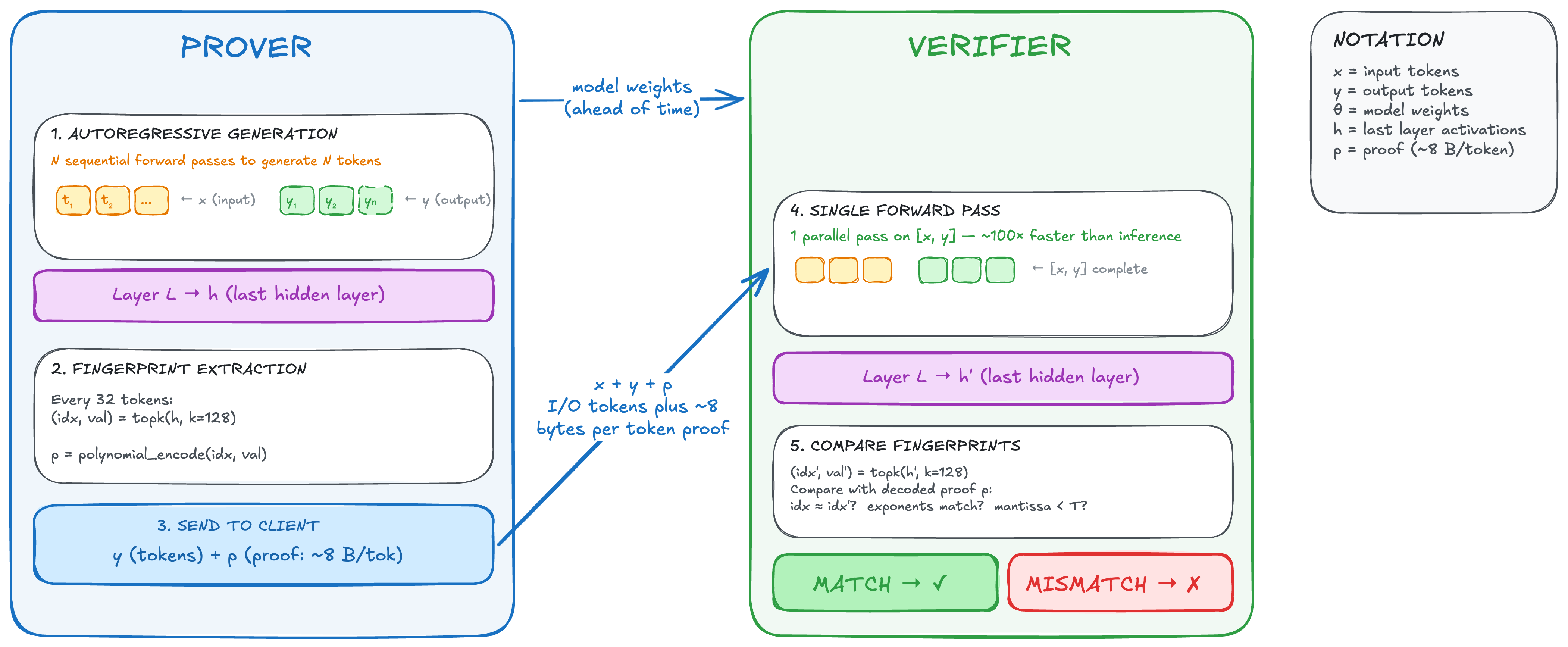
2. The prover performs inference with model M run on input tokens x to produce output tokens y.
3. For a subset of tokens, the prover records the 128 largest-magnitude activation values and their indices from the last hidden layer (top-128 is a configurable parameter) and compresses them into a compact representation — the proof.
4. The prover sends x, y, and the proof to the verifier.
5. The recomputation server independently re-runs M over the full sequence (x followed by y) in a single forward pass and reads off the same top-128 last-hidden-layer activations.
6. The recomputation server performs the same compression of its recomputed activations and checks this against the prover’s proof. It does not require an exact match: it accepts only if the differences all stay below preset thresholds.

The last hidden layer activations — specifically the high-magnitude values — are chosen as the comparison because they are stable enough across different hardware and numerical implementations, but sensitive to any change in the model or input. The encoding is compact: ~8 bytes per token, adding negligible network traffic to the verifier.

Changing the threshold will significantly affect the range of deviation between prover and verifier that is accepted, potentially opening a door for prompt-based attacks (steganography, etc.). Finding good threshold values is a key part of operating TOPLOC and may need to be performed for each model by the verifier.

Token-DiFR (inference verification)

The scheme outlined here was proposed in the DiFR paper.

1. Model M is loaded onto a secure recomputation server that the verifier operates inside the prover’s data centre.
2. A seed is shared between the verifier and the prover (dictated by the verifier). This seed is used to make the pseudo-random token decoding (selection) algorithm exactly the same between the verifier and prover.
3. For each token sequence, the prover sends the prompt x and generated sequence y to the verifier. The verifier then computes a single token using the same model M, temperature settings, etc. and extracts the logits for each token in the sequence.
4. The verifier calculates the “logit difference” (using the shared settings for temperature, top_k, etc.). The logit difference is zero if the tokens match exactly, and gives an idea of the “closeness” if the tokens do not match exactly. A large logit difference indicates that the model, settings or input may have diverged.
5. The logit difference is averaged across each token in the sequence, to give an overall deviation score. Lower score = more likely to be the same model and setup.

We have a prototype system that runs Token-DiFR on various models that we are testing now — see a future tech note for our results.

Pre-Training

This scheme is based on the schemes presented in Proof of Learning (2021) and Checkmate (2025).

To verify that the prover is running the declared pre-training workload, the verifier will re-run some of the training steps (producing Z_t from Z_t−1) of its choosing and compare outputs.

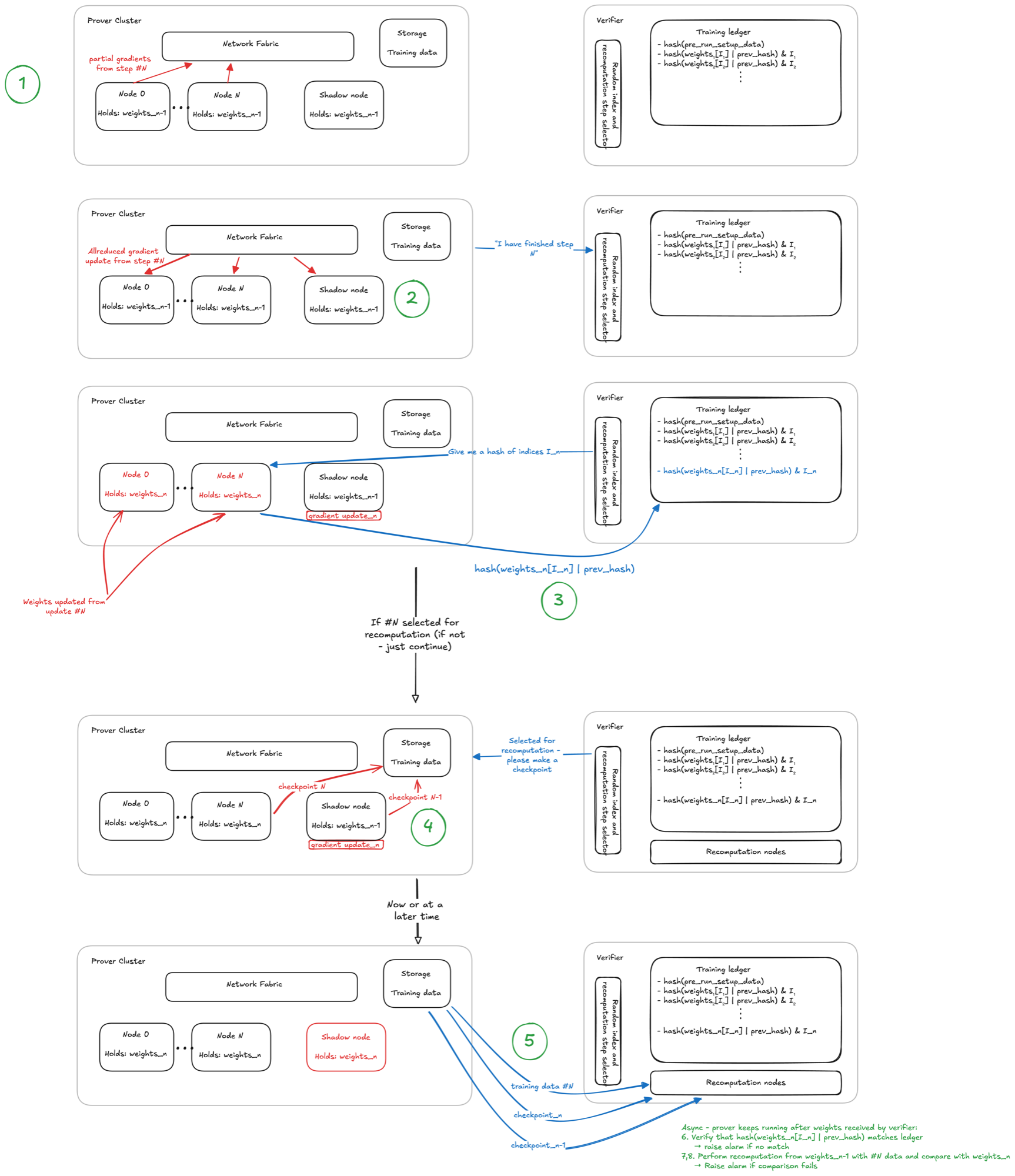
Re-running a step needs the model’s full training state — weights, optimizer state, and seed — at that step (a “checkpoint”). The verifier therefore needs the starting checkpoint (Z_t−1) of the model for any training step it attempts to verify. However, so that for every training step there is a credible threat that this step could be verified, the verifier must get to decide when checkpointing occurs and the step must have finished before the prover knows if it’s being recomputed or not.

Taking a checkpoint at every step imposes a large performance penalty on the prover, as writing a checkpoint to storage takes significantly longer than the step itself (>100% overhead). To avoid this a shadow node is used to store a buffer of the Z_t−1 checkpoint. Specifically, it is a spare data-parallel replica given no data to train on; each step it simply receives the same averaged (“AllReduced”) gradient the training GPUs already exchange, and applies it.

The verifier may also be concerned about whether the prover trained the model itself and didn’t just steal one. To prevent this, the prover must share the initialisation strategy from a pre-agreed set. The verifier checks whether the shared initialisation distribution of the weights then is sufficiently likely to have come from this initialisation strategy with a statistical test (Kolmogorov–Smirnov).

At every step:

1. The prover runs training, producing state Z_t.
2. The shadow node’s copy of Z_t−1 is updated using the gradient update calculated from backpropagation on the other nodes (specifically using the AllReduced gradient).
3. To ensure that when the verifier proceeds to a recomputation step the prover can’t quickly create a self-consistent Z_t, Z_t−1, and D, the verifier takes a small sample of the weights at each step. They name a few random positions I_t within the weights, the prover appends these to the previous entry’s hash, and then commits a hash of (Z_t[I_t] | prev_hash) to the ledger — before it learns whether step t will be audited. With the fingerprint committed first, the prover cannot later doctor the checkpoint to pass; and chaining each entry to the one before makes the ledger a tamper-proof, in-order history.

On steps randomly selected by the verifier:

1. The prover saves the checkpoint at t (using the training cluster) and t−1 (using the shadow node).
2. The prover shares checkpoints Z_t−1 and Z_t and the data D used for training step t (from cold storage).
3. The recomputation node confirms that the shared checkpoints and the data batch match their committed fingerprints in the ledger.
4. The verifier’s recomputation node performs a training step on Z_t−1 using D to produce Z′_t. This occurs slowly as the verifier does not have the same parallelism as the prover.
5. The verifier compares its Z′_t against the prover’s Z_t checkpoint, accepting if they agree within a calibrated tolerance.

A necessary pre-agreement: verifier’s frequency of checking. As checkpointing is a standard part of training, but the verifier gets to call when it occurs, the verifier and prover need to agree to a reasonable rate.

Appendices

1. Completeness

We have not discussed how the completeness claim is verified. There are attacks on the schemes above that involve running hidden workloads on the same compute, and substituting work. This is not in scope here, but is very important! Mechanisms to verify completeness will be discussed in a separate post.

2. Non-determinism

Breakdown: fundamentally, computers are deterministic, except for cosmic rays causing bit flips, though this is largely mitigated by ECC (error-checking code) memory. The main causes of “non-determinism” are:

1. Intentional randomization — e.g. the starting weights are intentionally randomised. This is done deterministically, using RNGs (random number generators) that have fixed algorithms and seeds used to generate the random numbers. These seeds are committed so that they can be replayed.
2. Floating point error. Floating point operations are deterministic! The issue is that they’re not associative, e.g. a(bc) ≠ (ab)c. There are some operations inside ML training and inference that reorder operations like this, often for optimisation. This can be done in response to some truly random thing, such as job scheduling on the GPU, and hence some floating point error exists in the final outputs.
   1. We deal with this by doing recomputation and using slightly fuzzy comparison — we don’t check byte-correctness but check closeness. Although a(bc) ≠ (ab)c, the two are very close to each other (otherwise floating points would be pretty useless!). There are some clever methods to choose comparison with the “most close” part of the things being compared. In the inference case, this involves intentionally choosing the largest N values to compare, as larger values suffer from less floating point error (TOPLOC).
   2. There are some others working on making the algorithms totally deterministic, so that training and inference can be byte-reproducible. This involves ensuring that operations that are mathematically associative (e.g. multiplication of real numbers) are always performed in the same order, or by gathering some extra data about the ordering or rounding performed (see arXiv:2403.09603).
3. Hardware generation. Even with identical code and seeds, training on A100s versus B200s can produce different results due to different hardware implementations of floating point units, different fused multiply-add implementations, and different tensor core behaviours. This is sometimes due to non-compliance with the IEEE floating point standard, or the standard not covering a specific operation (e.g. BF16 is not in the IEEE standard).

3. Practicalities

The prover and verifier would need to agree on a mean rate of checkpoints, plus any hard limits, e.g. “on average every 1000 steps but not slower than every 2000”. We can’t enforce a lower bound as this gives the prover known steps that they can cheat on.

4. Efficiencies

The hash commitment of every step could also include some optional non-hashed values that allow the verifier to cheaply sanity-check the training trajectory — for example, confirming that the loss is decreasing in a pattern consistent with the committed learning rate schedule, or flagging anomalous gradient norms that might warrant closer inspection:

• loss (optional) — how wrong the model’s predictions were on this batch
• gradient norm (optional) — magnitude of the weight update applied this step
• learning rate (optional) — scaling factor applied to the weight update

5. Future proofing

ZeRO-3 is a memory optimization strategy where each node does not contain a complete copy of the training data, only a shard of it. In this regime, an Allgather operation is used to compute passes layer by layer, so each node has a copy of each layer at some point in the step (which is then discarded for the next layer). The shadow nodes should be able to extract each layer in this way and build up a complete set of training data for each step.

We believe that in most cases there will be many data-parallel replicas, with ZeRO-3 used at one level below this. This needs confirmation.

6. Probability of being caught cheating

The recomputation will take many training steps to complete, because the verifier’s compute is much slower than the prover’s.

The verifier needs to be able to credibly threaten to recompute any step — otherwise the prover can cheat on steps that they know won’t be recomputed. The verifier needs to threaten recomputing a step even while they are already running a recomputation. A nomination during a recomputation cancels the currently running recomputation to start the new one.

The verifier needs to set the recomputation-choosing rate so that this aborting is uncommon. In the limit of high cost for being caught, the prover does not cheat if there is a credible threat on every step.

More rigorously, given probability p of each step being recomputed, the probability of a step being successfully recomputed is

q = p(1 − p)^k, where k = T_recomp / T_step

and k is the number of training steps that recomputation takes. This is the probability that the step is chosen for recomputation — p — times the probability that the recomputation is not interrupted by another recomputation — (1 − p)^k.

q is maximal when p = 1/(1 + k). For large k, this is ~1/k. If recomputation takes 1000 times longer than each step (k = 1000), then the verifier should set p to be 1/1001 ≈ 0.001.

It’s important to point out that q is strictly larger if k is smaller.

Note: there may be better strategies for the verifier’s sampling to increase the probability of catching cheating. The probabilities are slightly complicated if there is a hard lower limit on checkpoint frequency.

Acknowledgements

The schemes here build directly on prior work. Credit for some of the underlying methods belongs to the authors of those works:

• Inference (TOPLOC) — our scheme is a variant of TOPLOC.
• Inference (Token-DiFR) — follows the DiFR paper.
• Pre-training — based on the schemes in Proof of Learning (2021) and Checkmate (2025).